Technical teams working in agroforestry, perennial crops, pasture, and row crops under canopy often ask: how can you quantify soil organic carbon with digital soil mapping when you can't see the soil?
People hear that digital soil mapping uses satellite remote sensing, picture a satellite looking down at bare ground, and assume that anything covering the surface (e.g., a canopy, a cover crop, crop residue) must block the measurement. From there it's a short step to the misconception that it only works when the soil surface is completely exposed, not in systems like theirs.
In reality, seeing the soil has very little to do with how digital soil mapping works. And rather than blocking our view, vegetation cover can provide useful information — the amount of vegetation aboveground is correlated with how much carbon enters the soil below.
Here's a thought experiment: Suppose a satellite could see bare soil every day of the year, capturing the shades of brown, beige, black, and orange shifting across a field through the seasons. Would that enable you to quantify the carbon underneath? It wouldn’t. The color of the surface tells you remarkably little about how much carbon is held in the soil below.
Quantifying soil carbon without ‘seeing the soil isn't new or unique to digital soil mapping. Biogeochemical models have estimated soil carbon for decades using climate, soil, and management inputs, without ever laying eyes on the ground. That’s because biological, chemical, physical and historical properties of the soil are the crucial ingredients for predicting soil organic carbon, and all of these are included in our digital soil mapping algorithms.
What digital soil mapping actually relies on
.png)
Digital soil mapping uses soil samples, machine learning, and biogeochemically-informed predictors to quantify soil organic carbon (SOC) at scale. It works by building relationships between biogeochemical properties that can be observed or modeled across space, alongside actual soil samples measuring SOC content. Those observable inputs include farm practices like cover cropping and tillage intensity, the presence or absence of crop residue, topography, soil type, and long-term temperature and precipitation.
For example, whether there's stubble left on a field after harvest tells you something about how that land is managed — and that, in turn, is correlated with the carbon measured in the soil. Digital soil mapping learns thousands of relationships like this from real samples analyzed in a lab, then uses them to quantify carbon in places that haven’t been physically sampled.
Importantly, the strongest signals aren't single snapshots. They come from watching how a place behaves over time — how its vegetation, moisture, and temperature change across seasons and years. A field's pattern of green-up and senescence, the timing of planting and harvest, the presence of a cover crop in the off-season: these time-based patterns carry far more information about soil carbon than any one image of bare ground.
As our Senior Agroecosystems Scientist, Mitchell Donovan, PhD, has explained it, each soil sample is like asking the soil a question: given the land use, vegetation, moisture, and temperature experienced by the soil over the years, how much carbon were you able to store? Ask that question across tens of thousands of samples and the model learns to predict how soil elsewhere would respond to similar conditions — without needing a continuous view of bare ground.
Whereas other approaches provide SOC estimates only where samples were taken, digital soil mapping can predict SOC and uncertainty at every location in your project. As Verra has put it, "Compared with traditional soil sampling methods, digital soil mapping allows for broader spatial coverage, improved spatial resolution and precision, and increased cost-effectiveness, among other benefits."
Working in a new crop or geography
A reasonable follow-up question: if the model is learning these relationships, how does it work for a new crop or a new region?
It starts with our foundational model, ATLAS-SOC Core. ATLAS-SOC combines machine learning with microbial and biogeochemically-informed predictors drawn from remote sensing and environmental datasets, calibrated against a large, proprietary library of high-quality soil samples. It learns the general relationships between environment, management, and soil carbon — relationships grounded in the chemistry and biology of how carbon cycles through soil, which are fundamental processes that hold across climates, soil types, and cropping systems.
The foundational model works everywhere. Without any samples from your project, it can give you a relative picture of how soil carbon varies across a field, a region, or a sourcing area — where it's higher and where it's lower. For some teams, those relative magnitudes are enough to guide decisions without precise absolute values.
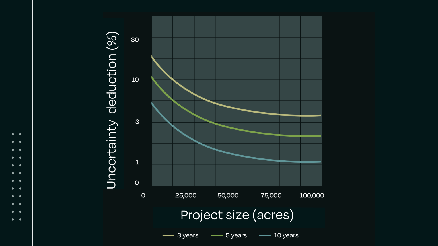
To align with a registry or claim removals in your Scope 3 inventory, you need more accurate estimates than those provided by the foundational model. For that, the model is localized — what we call ATLAS-SOC Fine-tuned. A modest set of physical soil samples from the project area is added to the calibration, so the model reflects your specific conditions and meets the accuracy those programs require. Grounding the predictions in primary data from your land drives uncertainty down — even compared to approaches that take more samples but make fewer predictions.
This process of fine-tuning the model on local project-specific samples, underpinned by a robust foundational model, is what enables digital soil mapping to work for new crops, land uses, practices, and regions.
——
Want to learn more?